[Update April 15, 2019] This blog post covers the 2018 course which you can find here.
TL;DR
The first lesson gives an introduction into the why and how of the fast.ai course, and you will learn the basics of Jupyter Notebooks and how to use the fast.ai library to build a world-class image classifier in three lines of Python.
You will get a feel for what deep learning is and why it works, as well as possible applications you can build yourself.
Introduction
These are my annotated notes from the first lesson of the first part of the Fast.ai course. I’m taking the course for a second time, which means I’m re-watching the videos, reading the papers and making sure I am able to reproduce the code. As part of this process I’m writing down more detailed notes to help me better understand the material. Maybe they can be of help to you as well.
Lesson takeaways
By the end of the lesson you should know/understand
- TL;DR
- Introduction
- Lesson takeaways
- Table of Contents
- The goal of fast.ai
- The practical, top-down approach of fast.ai
- How to use fast.ai
- Fast.ai Part 1 course structure
- How to run Python code in Jupyter notebooks
- Why we need a GPU and where to access them
- How to build your own classifier using the fast.ai library
- What deep learning is and why it works
- Digging a little deeper: The basics of Convolutional Networks
- The goal for this lesson
- Notebooks used in the lesson
- Interesting links / Links from the lesson
Table of Contents
- TL;DR
- Introduction
- Lesson takeaways
- Table of Contents
- The goal of fast.ai
- The practical, top-down approach of fast.ai
- How to use fast.ai
- Fast.ai Part 1 course structure
- How to run Python code in Jupyter notebooks
- Why we need a GPU and where to access them
- How to build your own classifier using the fast.ai library
- What deep learning is and why it works
- Digging a little deeper: The basics of Convolutional Networks
- The goal for this lesson
- Notebooks used in the lesson
- Interesting links / Links from the lesson
The goal of fast.ai
Fast.ai tries to achieve these three goals:
- Get you up and running with deep learning in practice,
- while delivering world-class results,
- using a coding focussed approach, without dumbing it down.
The practical, top-down approach of fast.ai
Most deep learning courses start from the bottom and work their way up, first explaining all the basic elements and then combining them. They make sure you understand the required linear algebra/math, non-linear functions, partial derivatives to then gradually introduce neural networks, much like most school/university courses are taught. This approach might have its benefits, it will take a long(er) time and a lot of perseverence to get to useful results.
Fast.ai uses a complete opposite, top-down approach by teaching you to create results right away and gradually introducing more and more of the concepts/details as you go along. Don’t worry, you’ll get to the nitty gritty details soon enough.
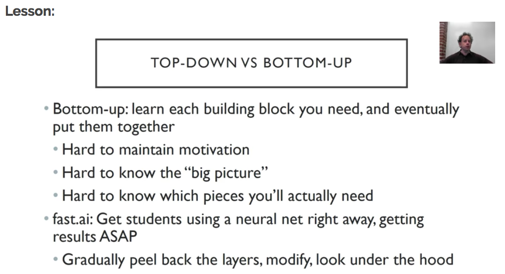
Think “whole game approach”: It is like learning baseball, you go to a game, learn to play bit by bit (and already enjoy), and later you can hone you skills and learn all the physics involved, instead of the other way around.
How to use fast.ai
The course is split into two parts:
each consisting of seven videos and a set of Jupyter notebooks (more on that later) to run the experiments and practice on your own.
The easiest way to watch the videos is on the fast.ai website. That way, you also have you easy access to both the course/lessons wiki as well as the general fast.ai forums to get help when needed or to discuss with fellow students.
You can learn a lot by watching the videos, but the better part of your time should be spent running and experimenting with the code, trying to reproduce and train your own networks. That is the only way to learn. I would, however, recommend you watch all the videos a first time and then go into more detail the second time around. As Jeremy explains in the lesson video, most students watch all the videos two or three times, while a second and third time around they also try to write the code themselves and start reading the mentioned papers. In my earlier review of the entire fast.ai course, I added a practical things section which discusses this in a bit more detail.
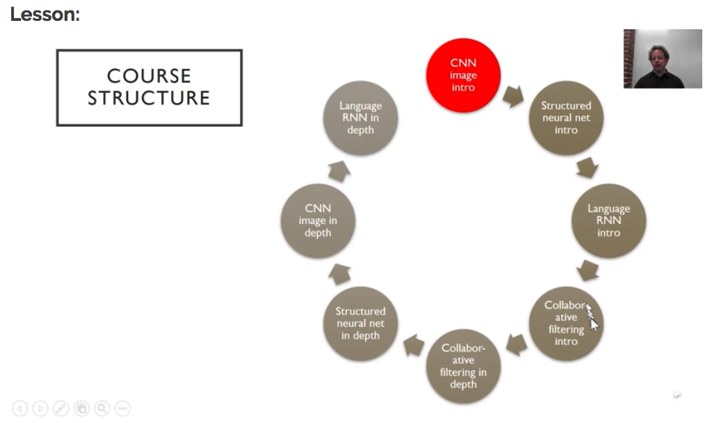
Fast.ai Part 1 course structure
This lesson is the first of seven in Part 1. The main goal is to get you up and running and train your first network, but don’t be fooled, there is a lot to absorb. Later lessons will cover structured data, language models and recommender systems in both an “intro” as well as an “in-depth” manner.
Let’s get started with setting things up.
How to run Python code in Jupyter notebooks
A lot of data science experiments are run using Jupyter notebooks which provide an interactive Python/markdown environment. We will discuss the basics of using Jupyter notebooks below and later on we will give some options to actually run them.
Jupyter Notebook basics
The Jupyter Notebook is an open-source web application that allows you to create and share documents that contain live code, equations, visualizations and narrative text. Although they are mainly used for Python development, there are a lot more languages supported if needed.
As we are most interested in running Python, for us, there are two main types of cells:
- Markdown for documentation
- Python code to run your experiments
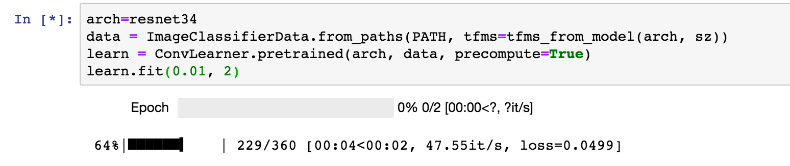
You can edit cells by clicking on them and using Shift+Enter to run the code inside, formatting the Markdown or running your Python code. Or you can use the menu at the top of the notebook:
While the cell is running, it has an ‘*’ indication to show it is still working:
The markdown cells allow you to add rich html documentation in between your code (snippets). If you are not familiar with Markdown, it is a text-to-HTML conversion tool for web writers and it is a great language to learn in general.
Python 3
It may sound a little stupid now, but when I started exploring deep learning, I had absolutely no idea which version of Python to choose. It is now safe to say that you should opt for Python 3 and never look back. :)
Jupyter Notebook shortcuts
Once you start spending more and more time in your notebooks, it is a no-brainer to learn the shortcuts for the most used actions you take, to keep you as productive as possible. Here is a list of shortcuts I use on a daily basis:
general shortcuts
Note: The Jupyter help menu shows all the shorcuts as a capital letter, but you should be using the lowercase letters:
| Command | Result |
|---|---|
| h | Show help menu |
| a | Insert cell above |
| b | Insert cell below |
| m | Change cell to markdown |
| y | Change cell to code |
Code shortcuts
When you are editing your Python code, there are a number of shortcuts to help you speed up your typing:
| Command | Result |
|---|---|
| Tab | Code completion |
| Shift+Tab | Shows method signature and docstring |
| Shift+Tab (x2) | Opens documentation pop-up |
| Shift+Tab (x3) | Opens permanent window with the documentation |
To open the documentation window or see the actual source code of the current method, you can simple prefix the code with ‘?’ or ‘??’ and run the cell.
| Prefix + run cell | Result |
|---|---|
| ?some_python_method | Opens permanent window with the documentation |
| ??some_python_method | Opens permanent window with the source code |
Notebook configuration
As you will see, each notebook will start with some specific commands which allow you to configure some settings. I always wondered what those where, I still can not write them off the top of my head, but I now know why they are there:
Reload extensions
%reload_ext autoreload
Whenever a module you are using gets updated, the Jupyter IPython’s environment will be able to reload that for you, depending on how you configure it (see configuration next or for more details).
Autoreload configuration
%autoreload 2
In combination with the previously mentioned reload extensions, this setting will indicate how you want to reload modules. You can configure this in three ways:
- 0 - Disable automatic reloading;
- 1 - Reload all modules imported with %import every time before executing hte python code typed;
- 2 - Reload all modules (except those excluded by %import) every time before executing the Python code typed.
matplotlib inline
%matplotlib inline
This option will output plotting commands inline within your Jupyter notebook, directly below the code cell that produced it. The resulting plots will then also be stored in the notebook document. For more info, you can read the docs here.
Why we need a GPU and where to access them
In order to train neural networks (more on those later), you will be needing a GPU (Graphics Processing Unit), which are already used to render video game graphics and more recently to “mine crypto-currencies”. Those same GPUs will help you train your deep learning models. At the moment, this requires an NVidia GPU, as those are the only ones that support CUDA, the language/framework that most deep learning libraries depend on to do their work. You ‘could’ perform the training on your CPU (Central Processing Unit) but that would take ages to complete for even small networks. More research is being done to train neural networks on any type of GPU, but for now we can only use NVidia ones.
Unless you own a gaming laptop or a serious/gaming machine, you most likely do not have access to a GPU. There are however, a number of options for you to try a GPU machine (and deep learning for that matter) at low cost.
Options discussed in the lesson video
Crestle.com provides (in their own words) an “effortless instracture for deep learning”, allowing you to create an account and start using Jupyter Notebooks in your browser. It has the lowest barrier to entry of the two options, but is a little bit more expensive (at the time of writing, so be sure to check yourself).
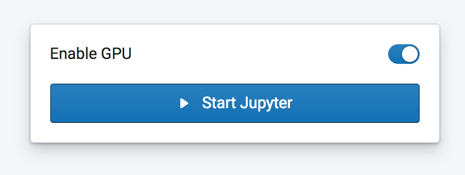
It is a little bit more work to get started using Paperspace, but you will have more options in configuring your machine including a selection of hard drive size and GPU type. More help and a coupon code to get started with Paperspace can be found on the fast.ai forums.
Some more options
Apart from the two options mentioned in lesson 1, there are plenty of options to run your Jupyter Notebooks in the cloud, below is a non-exhaustive list:
Run Notebooks from Github, Google Drive or start with some examples, the choice is yours. You even get 12 hour of free training time. The downside I experienced was the GPU memory was quickly filled, eventhough they have 12GB of RAM (ymmv), as well as having to re-run your code when the session is terminated (including installs and data downloads). But hey, it’s free!
Azure Notebooks preview provides free Jupyter notebooks for your deep learning experiments. However, at the time of writing, they are not providing GPU support to train your models. But as this is a preview, that functionality might be added soon enough.
- Localhost or any cloud provider
Obviously, if you have a machine with an NVidia graphics card at home or in the cloud, you can simply run the fast.ai notebooks on it. You can use this install script to prepare your machine. Here are the basic steps you need to run (the script might need changes for your specific setup though):
$ wget http://files.fast.ai/setup/paperspace
$ chmod +x paperspace
$ sudo ./paperspace
These steps include cloning the fast.ai GitHub repository and installing all required packages.
My personal experience
Personally, I started out with both Crestle and soon thereafter Paperspace, and then switched to an Ubuntu VM hosted on Azure. I might get my own machine one day, but for now I’m just running it in the cloud. There are, however some things I have learned that might be of interest:
-
jupyter notebook --no-browser
In every single video I have watched, everyone starts their notebook in the following way:
$ jupyter notebookHowever, when I do that, I get the following message:

I fixed this by starting my notebooks with the following command:
$ jupyter notebook --no-browserIf you have a better solution, feel free to let me know… :)
-
Secure access via port forwarding
When running your Jupyter Notebooks on your own server, you need to find a way to securely access it. The Jupyter documentation spends a complete chapter on securing your notebook server, but if you are running it only for yourself and have ssh access, using ssh port forwarding might save you some headache and keep you running secure:
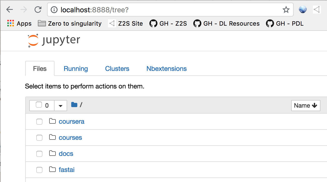
# ssh -L local_port:remote_host:remote_port remote_machine_ip
$ ssh -L 8888:localhost:8888 my_vm_ip
This command will map your local 8888 port to localhost:8888 on the remote machine, allowing you to securely connect to your server in the following way:
-
Tmux (or Screen)
If you connect to a remote server to run your Jupyter notebooks (or any remote session, really) there is always a chance that your secure connection gets interrupted and your session gets destroyed. If you have been training your model for a couple of hours/days, that is not something you would like to experience.
An easy way to overcome this, is to run Tmux once you log in. Tmux will allow to manage (create, attach, destroy) different terminal sessions on your remote machine. If your connection gets interrupted, you can simple reconnect to the remote server and “re-attach” to terminal session that will still be running.
The easiest way to do that is:
# 1. On the remote machine run
$ tmux
# a new shell will open

# 2. In that new shell you can

# start your notebook
$ jupyter notebook --no-browser

# split your window
Ctrl+b + %

# switch between panes
Ctrl+b + o
Note that this post is not an introduction to Tmux but we are mentioning it here because of the absolute value it brings you. For a quick reference of useful commands check out our snippets repository on GitHub.
How to build your own classifier using the fast.ai library
Our first network will be able to categorize an image it has never seen as either a ‘cat’ picture or a ‘dog’ picture. To do that, we need three things:
- the fast.ai library;
- a labeled dataset;
- learn/train a neural network to distinguish between cats and dogs.
fast.ai library
The fast.ai library is a small Python library that will help us build world-class neural networks, based on three key elements:
- it implements all the best practices in deep learning (they could find)
- experiments with new papers that come out to see what works
- built on top of PyTorch, Facebook’s deep learning framework, which is heavily used in research/academia, as opposed to Tensorflow from Google, which is another very popular deep learning framework. For more deep learning frameworks, have a look at our deep learning resources on Github.
The fast.ai library is an abstraction on top of PyTorch, but even more so than Keras over Tensorflow imho. The fast.ai library offers a kind of application abstraction with some interesting helper methods, whereas Keras is a functional abstraction over a low(er) level API. If you start to dive in, it is sometimes challenging to understand how and why something works. The fastai doc project was created to address these issues and I hope to see this progress over the coming months.
A labeled dataset
To train our first model we will use a dataset containing labeled images of cats and dogs. This approach is called Supervised Learning. Based on the labeled images we provide, the network will learn to distinguish between cats and dogs.
The dogscats dataset consists of 23000 training images (50-50 split between cats and dogs) and 2000 validation images (same 50-50 split). Below is a picture of the folder structure of the dataset:
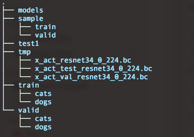
The “train”, “valid” and “test1” folders contain the training, validation and test images respectively. Both the training and validation folders have a subfolder for each label we want to train/categorize on, each containing images that should be classified according to that label. Important to remember is that a lot datasets are structured this way.
Why is the data split this way? When I started with deep learning, it took me a while to get a hang of what exactly the difference was between those three (sub-)datasets. When you train a network, you will usually try multiple configurations/parametrizations of that network, to see which configuration works best. In order to do that you will need a training and a validation set:
- Training set: The data used to train a specific configuration of a network;
- Validation set: The data used to validate different configurations of a network.
Once you have found and trained a network that seems to perform to your liking, you use the:
- Test set: The data used to evaluate the network’s performance as a whole.
It is important that none of the information from the test set, is used to train/validate the network. There is a good blog post of the fast.ai site diving a little bit deeper on this topic or have a look at the fast.ai machine learning course.
One other interesting folder is the “model” folder, which will store the versions of your model you save. These saved models will be used to deploy your solution to production.
Side note: Getting the data - PDL - Python Download Library
While working with the fast.ai (and other) notebooks, you typically download some type of dataset (file) and store it locally to use for training and validation. You can get those files using a tool called “wget” or download them via your browser and unzip them to your file system. While always downloading, unzipping and moving those datasets, I decided to create a small library to keep me from ever having to wonder about that again, and so, PDL (Python Download Library) was born. It is a small Python library that eliminates the hassle of getting your data where it needs to be. Additionaly, I have started adding common datasets to the api, so you can provision the data with a simple method call (see below).
If you want to know more about downloading datasets, or running bash code/scripts in your Jupyter notebooks, check out the blog post on downloading datasets and an introduction to PDL or have a look at the PDL source.
You can simply install it from the command line
$ pip install pdl
or in your Jupyter notebook:
!pip install pdl
Once installed, you are good to go. For more details, have a look at the documentation.
from pdl import pdl

pdl.catsdogs()

# or

pdl.download("https://some.url.com/")
Important Note: we are very fortunate to have a dataset that is already prepared for us to use in training. Once you start to experiment with your own ideas, you will learn that availability, accessibility and quality of data can be a challenging task.
Explore a data sample
Having the data in place, it is time to explore and get a feel for the data. Try to understand what is your dataset by exploring some images, it will help you configure your network to gain better results. After training and testing, have a look at images your model got right/wrong, so you can improve further.
We will have a look at one sample from our dataset. The picture below shows us how most people see the image displayed by the computer. It is a black cat lying on some furniture, with green flowery wallpaper and some cans in the background. It is 278 pixels high and 375 pixels wide.
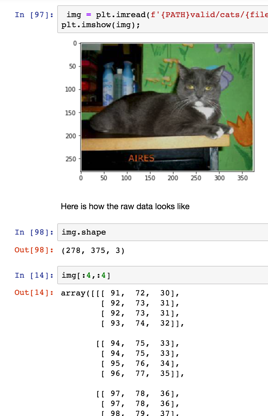
Computers, however, do not see the picture the same way we do. If we look at the image shape, we see there is a third dimension, namely “3”, this represents the Red-Green-Blue (RGB) dimension. So, for each pixel, we have three values, one for red, one for green and one for blue. So the picture array consists of three values (RGB) for each pixel in the 278x375 image area. At the bottom of the picture above, we show the top 4x4 pixels of the image, all these numbers are between 0 and 255. We will use these numbers to train our network later on.
If you are already running your notebook, you can experiment with this part of the code until you fully understand what is going on - which is probably what you should do for all the code you run :).
Train our first network
Having acquired and explored the training data, it is time to train the our network. What is remarkable about the fast.ai library, is the amazing simplicity of how you can achieve that and with such accuracy; here is the code:
from fastai.imports import *
from fastai.transforms import *
from fastai.conv_learner import *
from fastai.model import *
from fastai.dataset import *
from fastai.sgdr import *
from fastai.plots import *
# Specify location of your data
PATH="data/catsdogs"

# Specify size each image will be resized to,
# you can start will a smaller size for faster training and enlarge from there
sz=224
arch=resnet34
data = ImageClassifierData.from_paths(PATH, tfms=tfms_from_model(arch, sz))
learn = ConvLearner.pretrained(arch, data, precompute=True)
learn.fit(0.01, 2)
architecture
Neural networks come in different shapes and sizes, and depending on how they are structured, their results tend to vary. Fortunately, you do not have to reinvent the wheel for every solution you wish to build. There are a number of architectures out there that have proven to be extremely successful, so we can reuse those for our own classifier. Using the fast.ai libary, we can indicate which architecture we want to use to train our network on, instead of having to build it all by ourselves.
Here we use “resnet34”, which has some “related” architectures some of which are also implemented in fast.ai, you can play around and see what results you are able to get:
- resnet18
- resnet50
- resnet101
- resnet152
Other architectures for image classification include:
- GoogleNet
- AlexNet
- VGG
- Inception v(1, 2, 3)
data
The “data” variable is used to configure our data for training. We specify where the data is stored (PATH) and apply the data transformations that come with our selected architecture (tfms_from_model). These transformations can vary for each architecture but usually entail one or more of these:
- resizing: each images gets resized to the input the network expects;
- normalizing: data values are rescaled to values between 0 and 1;
\begin{aligned} y = \frac{x - x_{min}}{x_{max} - x_{min}}\end{aligned}
- standardizing: data values are rescaled to a standard distribution with a mean of 0 and a standard deviation of 1;
\begin{aligned} y = \frac{x - μ}{σ}\end{aligned}
where μ is the mean and σ is the standard deviation.
learn
We create a learner object to train our network on the data using the architecture we selected above. An additional benefit to using a pre-existing network archicture, is that it usually comes with a pretrained model, meaning the architecture has already been pretrained a massive dataset (e.g. ImageNet). This way we do not start training from zero (or some random initialization) but we start from a model that already gives good results, and adapt it to fit our specific needs. This is method of learning is called Transfer Learning.
learn.fit()
Once we have our data and learner in place, we can start the actual training, which is done by the fit(learning_rate, epochs) method that takes two parameters. The first one is the learning rate and it is used to update our model during training, it is a measure of how fast we want our model to learn. Setting a low value will gives good results, but implies a long training time; setting a high value will allow us to train much quicker, but we might overshoot our goal. Below, we discuss the learning rate and how fast.ai helps you pick a good learning rate for your model in more detail.
The second parameter is the number of “epochs” we will train for. An epoch is one cycle where our model sees every image in our dataset once. The question of how many epochs you need, can simply be answered with “as many as you like, as long as the accuracy of the validation set keeps improving”. Sometimes, if you have a really big model, you might limit the number of epochs based just on the time you have available.
Try it yourself
In the lesson video and your Jupyter Notebook you can train the model and validate its results. A good way to validate if you understood everything up to now, isto train your own network on some data you can find. Examples:
- euro/dollar bill classifier;
- boat, car, plane classifier…
Some questions you should try to answer:
- How many images do you need to get good results?
- How do results/training time vary using a different learning rate?
- How do results/training time vary using a different number of epochs?
What deep learning is and why it works
Why we classify
We just finished building our first image classifier. If you are now wondering what is so interesting about an image classifier, it might be a good time to see where they are being used.
AlphaGo
Chances are you have heard of AlphaGo beating the world champion at Go. It used an image classifier to train the computer to learn what good/bad Go board looked like, which is key in learning how to make a good next move.
Fraud detection
One of the examples mentioned in the lesson uses an image classifier for fraud detection. By turning browser mouse movements into heat maps, the image classifier was trained to identify fraudulant users and/or bots.
Artificial Intelligence > Machine Learning > Deep Learning
Merriam-Webster defines Artificial Intelligence as:
- a branch of computer science dealing with the simulation of intelligent behavior in computers;
- the capability of a machine to imitate human behavior.
Arthur Samuel coined the term “Machine Learning”, while he was teaching a main frame computer to play checkers against itself to learn a good/the best strategy. Machine Learning can be described as a program that is able to learn a certain task from experience. However, traditional machine learning can be difficult as well as knowledge/time consuming.
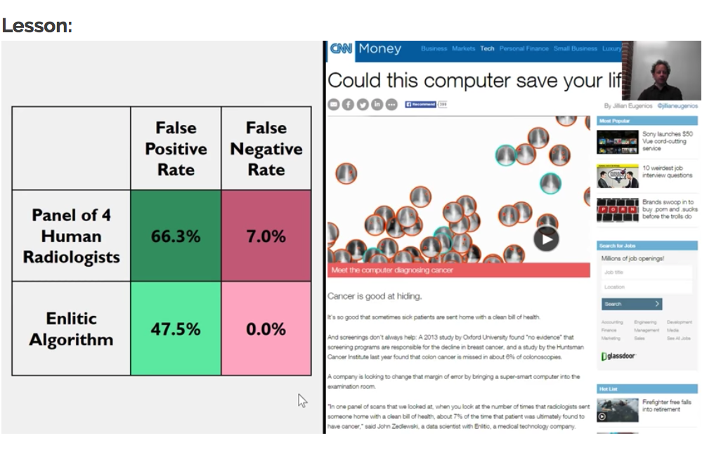
Let us look at the example of the “Computational Pathologist” (CPATH). The idea was to create a computer program that could outperfom a human pathologist in analyzing patient scans. It was created by taking a lot of pathology scans and examinening them together with a lot of trained pathologists to discuss what could be relevant features (aka manual feature engineering), and they came up with specialist algorithms to calculate those features, which in turn where then passed to a logistic regression (classification). Although the results were very good, this approach took a lot of domain and computer science expertise, not to mention many years of work.
From the previous example it is easy to see, that if we want to apply this method to a larger, complexer and more diversified set of problems, we will need something better. Therefore, we will try to explore something a bit more flexible:
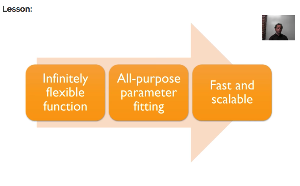
Let’s look at each of these:
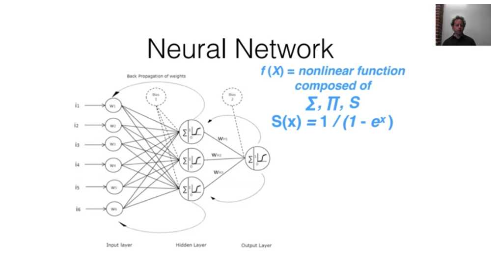
Infinitely flexible function: A neural network
The underlying function that deep learning uses, is called a neural network, which will be implementing later on.
What we need to know at the moment:
- a set of simple linear functions
- combined with a set of simple non-linear functions.
When we combine them in this way, we get something called the “Universal Approximation Theorem”, which states:
This kind of function can solve any given problem to arbitrarily close accuracy, as long as you add enough parameters."
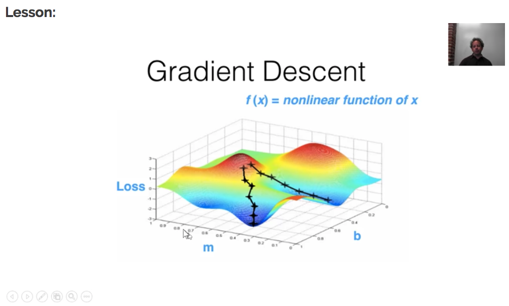
All-purpose parameter fitting: gradient Descent
The way we fit the parameters from our neural network is a technique called “Gradient Descent”, which in essence works like this:
- how good are my current parameters?
- figure out a slighty better set of parameters;
- follow the surface of the “loss function” to find the minimum.
The “loss function” - aka cost function, error function, objective function, criterion - is a metric for how far off we are with our predictions using the current set of parameters.
Looking at the picture below, you see that depending on where you start (= the initial parameters you start with), you end up in different places, different local minima. But, it turns out that, for neural networks there are different parts of the space that are equally good. Or to say it in another way, in the context of deep learning, we generally accept such solutions even though they are not truly minimal, so long as they correspond to significanlty low values of the cost function. (“Deep Learning”, Ian Goodfellow et al.).
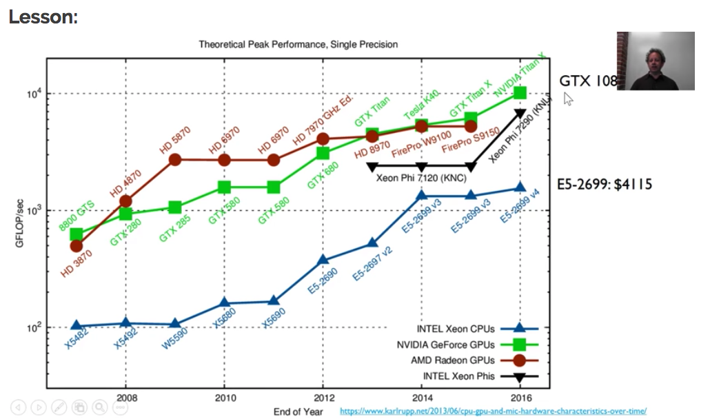
Fast and scallable
Fitting the parameters using Gradient Descent is a computationally intensive process and we need to do this in a “reasonable amount of time”. It is really only thanks to the advancements in GPU power and vectorized implementations, that we are able to use these kinds of networks. The graph below shows the evolution of CPU vs GPU power evolving over the years, whereas the top GPU mentioned in the graph is also a couple of times cheaper than the best CPU.
Side note: Why now
In general, three technical forces are driving advances in machine/deep learning:
- Hardware
- Datasets and benchmarks
- Algorithmic advances
If you want to read a more detailed discussion on each of these three, I would recommend “Deep Learning with Python” from Francois Chollet - start reading at page 20, which is the best explanation of these advances I have come across so far.
One more thing
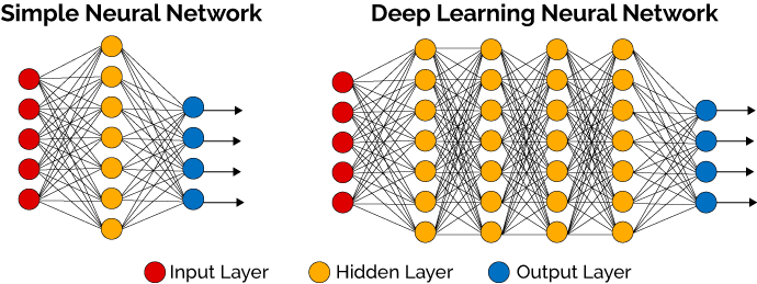
Although the example neural network (with one hidden layer) supports the universal approximation theorem,
it requires an exponentially increasing number of parameters to do so, meaning they do not actually solve the fast and scallable for even reasonable sized problems. But, if you add multiple layers (see image below), you can get super linear scaling. You can add a few more hidden layers, to get multiplicatively more accuracy to multiplicatively more complex problems. This is what is called Deep Learning: neural networks with multiple hidden layers.
 (Picture from KDnuggets - deep learning made easy)
Putting it all together: examples of deep learning
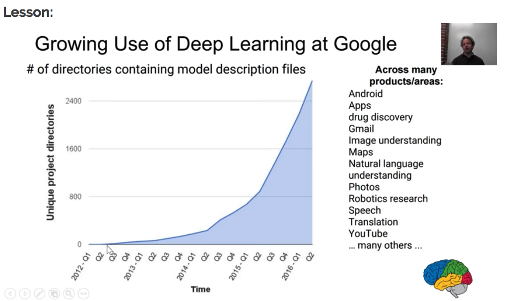
As of 2012, Google started investing more and more in deep learning. Below you see an overview of the growing use of deep learning at Google, note that the graph only goes up to Q2 of 2016.
Additionally, they also acquired DeepMind which is doing tremendous work in deep learning and reinforcement learning research/applications. Have a look at their website to explore the amount of awesome research they have been doing. Some examples of their work:
-
AlphaGo: the first computer to ever beat the world champion at Go, a board game which requires computers to be intelligent as it is too complicated to brute force your way to victory. Actually, AlphaGo already has a successor with the name of AlphaGo Zero, which learnt to play the game of Go simply by playing the game against itself, starting from complete random play. This type of learning is actually called “Reinforcement learning”, where an agent learns from its own state and surrounding environment to maximise its rewards by taking actions, and by doing so learns to perform a certain task.
-
Generative Query Networks - GQN: in a recent publication, they introduce the concept of a Generative Query Network, a framework within which machines learn to perceive their surroundings by training only on data obtained by themselves as they move around. Practically, it has been used to generate 3D environments from a single 2D photo.
-
There is a lot more examples on their website.
Google Inbox also used deep learning to provide suggestions for quick replies to emails, based on understanding the message content of the incomding email.
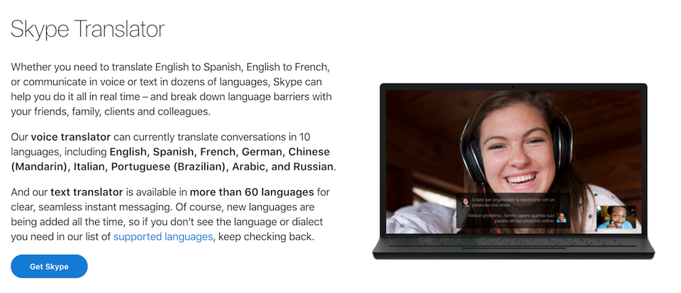
Microsoft Skype translation is out of preview and can translate conversations in 10 languages in real time.
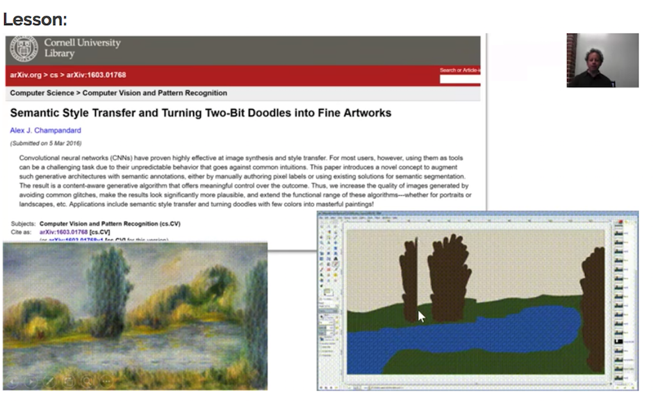
One particularly cool example is the Neural Doodle application, which is a kind of assisted deep learning that lets you doodle around to then generate an image based on a particular style.
Jeremy Howard, one of the co-founders of Fast.ai, also founded Enlitic, which is a deep learning long-diagnosis startup trying to make doctors faster and more accurate.
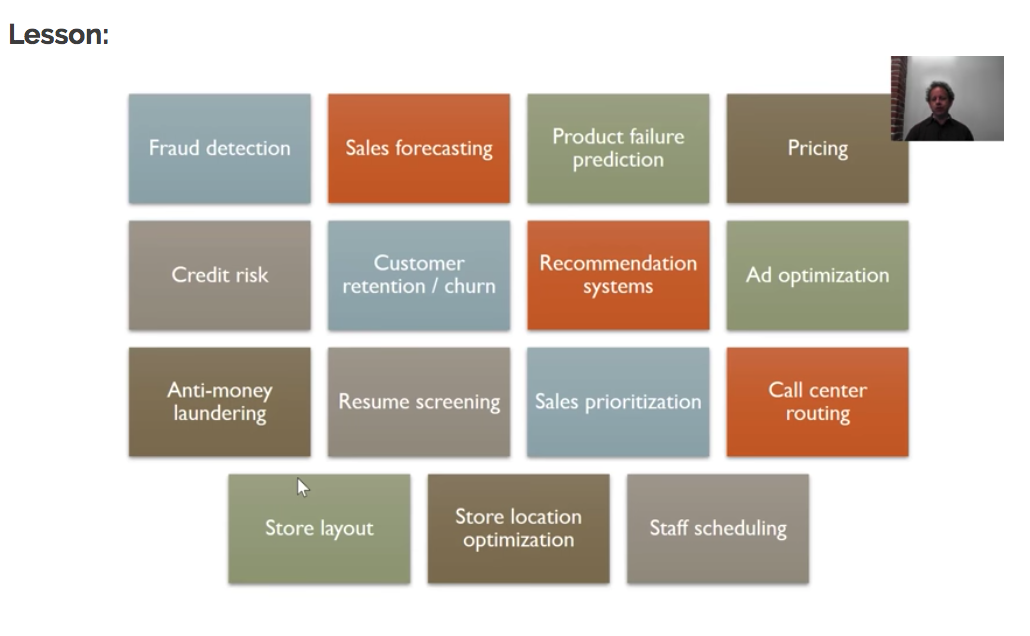
Finally, a general overview of some possibilities to try and apply Deep learning for:
Digging a little deeper: The basics of Convolutional Networks
What actually happened when we trained our image classifier?
With the code we wrote using the fast.ai library, we created what is called a “Convolutional Network”, convolutional neural network or CNN.
It is a specialized kind of neural network for processing data that has a known grid-like topology. Examples include time-series data, which canbe thought of as a 1-D grid taking samples at regular time intervals, and image data,which can be thought of as a 2-D grid of pixels. Convolutional networks have beentremendously successful in practical applications/
“Ch 9: Convolutional Networks - Deep Learning”, Ian Goodfellow, Yoshua Bengio and Aaron Courville.
Remember from before that for deep learning to be effective, we needed an infinitely flexible function where we could apply an all-purpose parameter fitting algorithm to, so I will discuss both of these here:
Infinitely flexible function
The hidden layers in a neural network contain both a linear and non-linear part in order to solve any problem to abritrarily close accuracy.
The linear part in a convolutional layer is called a “convolution” (or kernel). In the picture below, you see an example of how a convolutional step works.
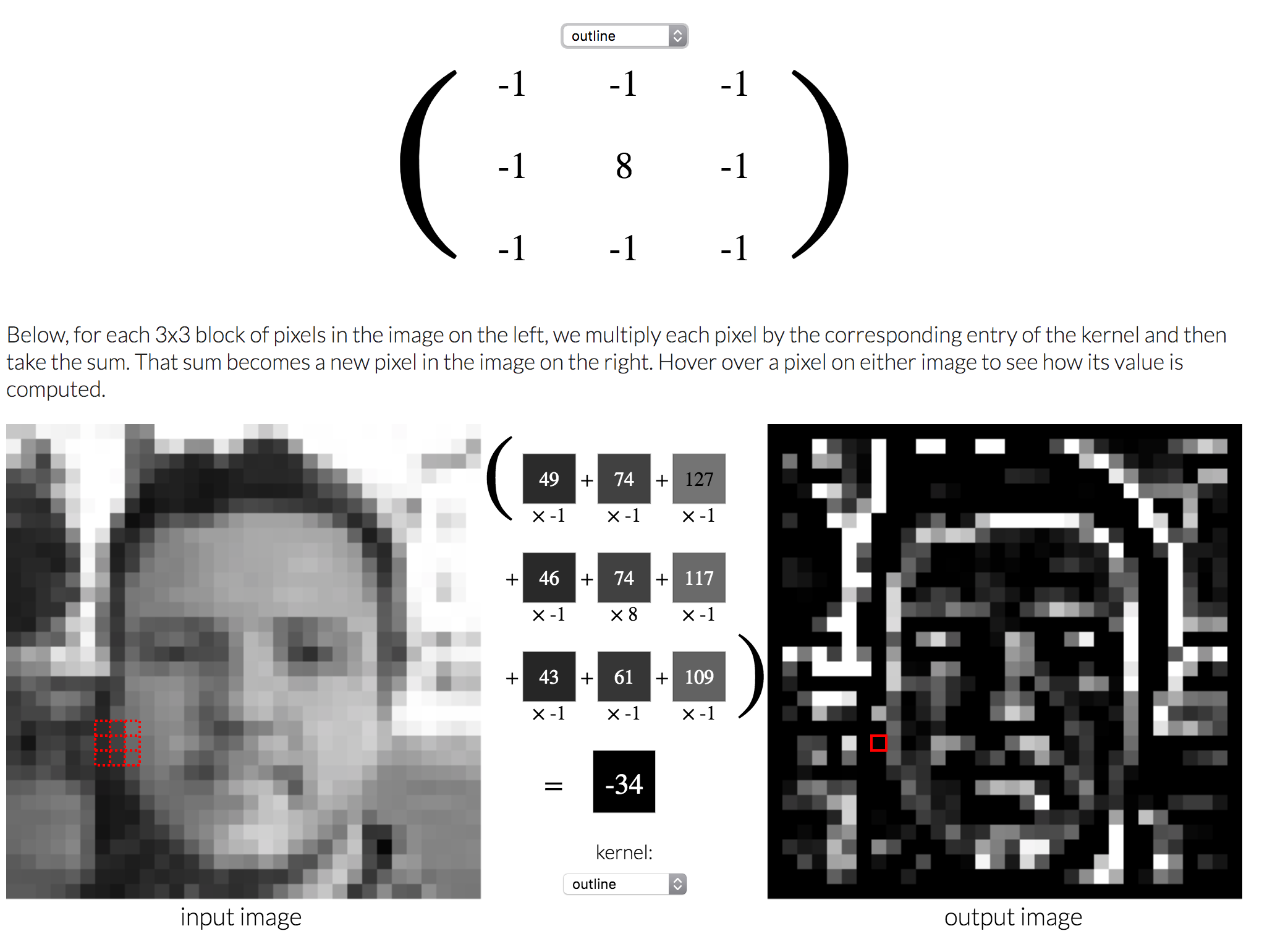
The input image on the left is transformed into the image on the right, by:
- moving a small “NxN” matrix/kernel (usually 3x3) over the input image;
- multiplying each pixel value in the NxN area with that matrix;
- summing up those values to get the resulting pixel value of the output image.
If you want to play around with it yourself, you try the excellent playground from Explained Visually.
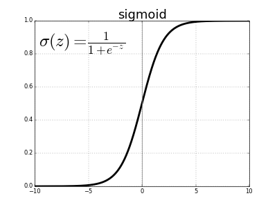
The non-linear part takes an input (from the convolution) and turns it into a new value in a non-linear way, which is what allows us to create arbitrarily complex shapes. To get a more in-depth reading on this, you can check out the amazing interactive “Neural Networks and Deep Learning” from Michael Nielsen. In deep learning, there are a number of non-linear functions used to achieve this:
- sigmoid function
\begin{aligned} \sigma_e(x) = \frac{1}{1 + e^{-x}} \end{aligned}
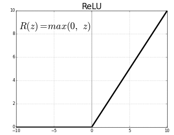
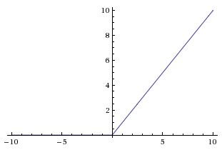
- ReLu (rectified linear unit)
\begin{aligned} ReLu(x) = max(0, x)\end{aligned}
- Leaky ReLu
\begin{aligned} LR(x) = max(\alpha(x), x) \end{aligned}
with α between 0 and 1.
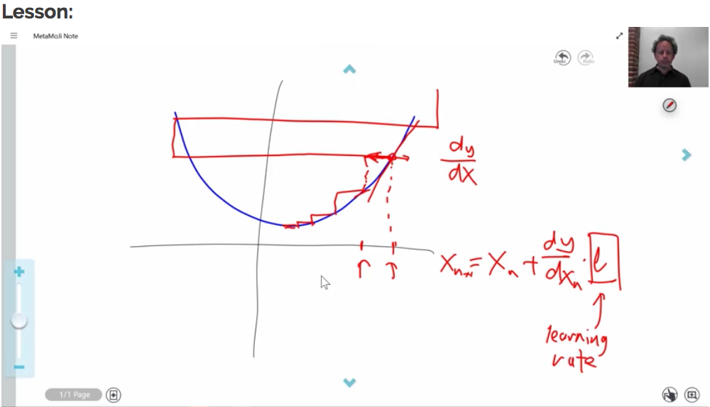
Gradient Descent and learning rate
Let’s say we want to get the minimum of a quadratic function using gradient descent. We start by calculating the value and the slope at point x. Next, we move a little bit down hill and calculate the value again. Once we see the value of the function is no longer decreasing, we can conclude that we are at the minimum. The size of the step we take to follow the slope downhill is called the learning rate. It is easy to see that by taking a small value for the learning rate, it would take forever to get to the minimum; taking a large value would give good results at first, but we might easily overshoot te minimum we are trying to reach.
Note: For quadratic functions we would never use this method in a real world scenario, but it is easier to get a feel for how it works for complex functions such as neural networks.
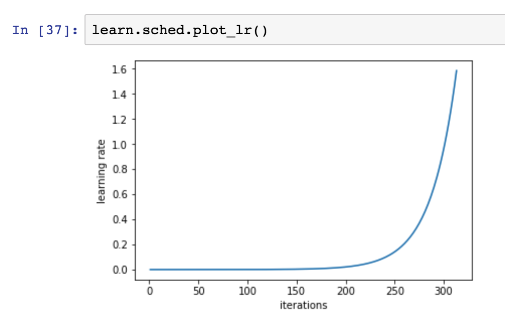
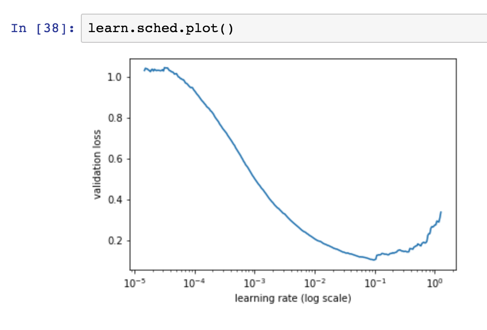
Now how do we select the “right” learning rate to start training our model? This question is a heavily debated one in deep learning and fast.ai offers a solution based on a paper from Leslie Smith - Cyclical Learning Rates for training Neural Networks.
The idea of the paper is quite simple:
- start with a small learning rate and calculate the loss;
- gradually start increasing the learning rate and each time, calculate the loss;
- once the loss starts to shoot up again, it is time to stop;
- you select the highest learning rate you can find, where the loss is still crearly improving.
Note: Earlier this year, he posted another paper related to setting hyper-parameters, which might be interesting: A disciplined approach to neural network hyper-parameters: Part 1 – learning rate, batch size, momentum, and weight decay
The fast.ai library has some great helper function to guide you through selecting a good learning rate:
# get a learning_rate from fast.ai
learning_rate = learn.lr_find()
# plot the learning rate over time
learn.sched.plot_lr()
# plot the loss function and see where it starts to increase again
learn.sched.plot()
Putting it all together
Looking at the convolution, non-linearity and gradient descent, it might be easy to miss the power these three rather simple elements give us. If we have enough kernels, with enough layers, something really interesting happens. The first layer(s) of the network learn basic building blocks of visual entities (horizontal lines, bits of sunset, circles…) and later layer start combining the building blocks from previous layers so that in three we learned to recognize text, wheels, presence of faces, and in even later layers we can recognize bycicles, animals…
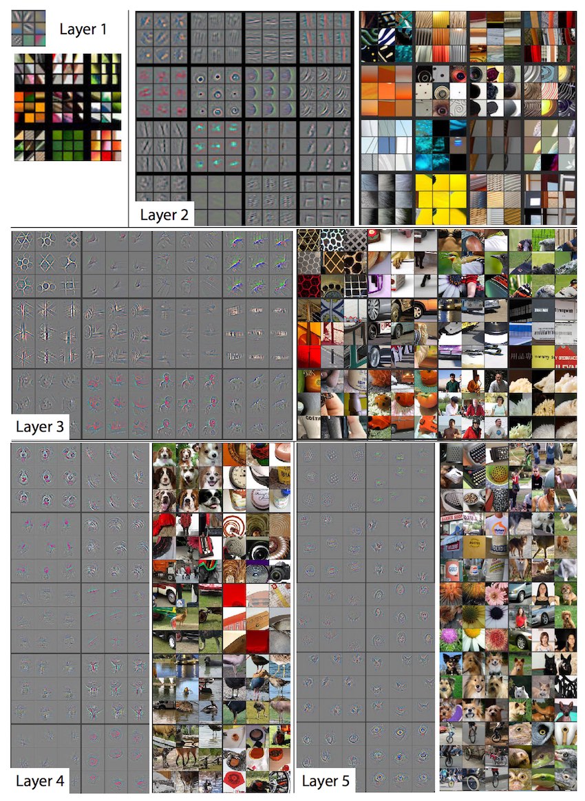
The visualizing and understanding convolutional networks paper gives a good idea of what actually happens in a convolutional network and how gradient descent learns the convolutional filter values over multiple layers.
The goal for this lesson
Make sure you can:
- run the code provided by the lesson1.ipynb
- apply/test your own dataset
- find some images online
- put them in the correct folders
- how many images do you need for each class?
- try to understand what types of images it works well for
- what kind of learning rate do you need for which types of images?
- how many epochs do you need
- get a sense of what is in the “learn” object
- make sure you can work with Numpy
- make sure you know the basis shortcuts to be productive in Jupyter Notebooks.
Notebooks used in the lesson
All the notebooks for the first part are located under courses/dl1/ directory. In this section we list the notebooks that are used in the session video:
Note that lesson 1 only goes up to “7 Improving our model”. The rest of the notebook will be covered in lesson 2.
Interesting links / Links from the lesson
- Fast.ai GitHub
- Cyclical Learning Rates for Training Neural Networks
- Visualizing and Understanding Convolutional Networks
- Fast.ai Mission
- Fast.ai Forums
- Jupyter Notebooks Project
- Michael Nielson - Neural Networks and Deep Learning
- How (and why) to create a good validation set
- Crestle
- Paperspace
- Azure Notebooks
- Google Colab
- Elastic GPUs Amazon AWS
- ResNet models
- PDL - Python Download Library